What Makes a Tick Tick?

Summarizing my work in UVM Honors Thesis Work.
Tick-borne diseases represent one of the most significant and rapidly escalating public health threats in the United States. With climate change projections suggesting dramatic shifts in temperature and precipitation patterns, understanding how environmental variables influence disease dynamics has become paramount. This honors thesis investigates the complex relationship between climatic factors and the prevalence of three major tick-borne pathogens within Ixodes scapularis populations across New England.
Research Background
The blacklegged tick, Ixodes scapularis, serves as the primary vector for multiple zoonotic diseases in the eastern United States, including Lyme disease (Borrelia burgdorferi), babesiosis (Babesia microti), and anaplasmosis (Anaplasma phagocytophilum). While previous research has focused on predicting tick population distributions under climate change, few studies have directly examined how temperature and precipitation affect pathogen prevalence within tick populations—a critical gap for understanding future disease risk.
Methodology
Site Selection & Field Sampling
Working with Dr. Ellen Martinsen and Dr. Nicholas Gotelli in the UVM Wildlife Pathogens Laboratory, I developed a novel approach to site selection using Principal Component Analysis of meteorological data from NOAA weather stations. This method identified four representative sites across New England’s climate gradients:
- Ashburnham State Forest, Massachusetts (n=38)
- Mountain Laurel Estates, Goffstown, New Hampshire (n=40)
- Jericho Research Center, Vermont (n=57)
- Saint Michael’s College, Winooski, Vermont (n=52)
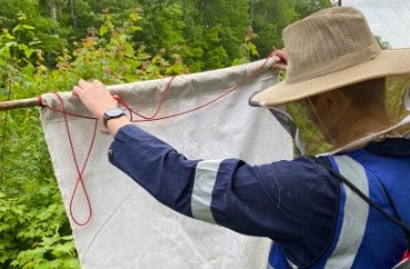
Adult ticks were collected between May and September 2023 using standardized drag cloth methods, with weekly revisits to each site until adequate sample sizes were obtained.
Molecular Analysis
Each collected specimen underwent multiplex PCR screening to detect all three pathogens simultaneously. DNA extraction was performed using the Qiagen DNeasy Blood and Tissue Kit, followed by gel electrophoresis to identify positive infections:
- B. burgdorferi: 550 base pair band
- B. microti: 310 base pair band
- A. phagocytophilum: 1200 base pair band
Key Findings
Pathogen Prevalence Rates
Analysis of 187 total specimens revealed striking differences in pathogen prevalence across the study sites:
- Lyme disease (B. burgdorferi): 73.2% average prevalence
- Babesiosis (B. microti): 3.7% average prevalence
- Anaplasmosis (A. phagocytophilum): 9.2% average prevalence
These results demonstrated statistically significant variation across sites (ANOVA: p = 2.433E-9), suggesting strong environmental influences on pathogen dynamics.
Climate-Pathogen Relationships
Multiple linear regression models revealed that temperature exerted a substantially greater influence on pathogen prevalence than precipitation across all three pathogens. The Lyme disease model showed particularly strong predictive power (R² = 0.98), while babesiosis and anaplasmosis models exhibited lower but meaningful correlations (R² = 0.18 and 0.45, respectively).
Key regression coefficients demonstrated:
- B. burgdorferi: β(temp) = 3.72, β(precip) = 0.003
- B. microti: β(temp) = -0.551, β(precip) = 0.0176
- A. phagocytophilum: β(temp) = 2.42, β(precip) = -0.0133
Climate Change Projections
2070 Disease Forecasts
By integrating our regression models with CHELSA v2.1 climate projections across three emission scenarios (SSP126, SSP370, and SSP585), we generated novel disease prevalence forecasts for the northeastern United States:
Lyme Disease Projections: Under high emissions scenarios (SSP585), our models project prevalence rates reaching 150 cases per 10,000 individuals by 2070—representing approximately 3 additional cases per county annually. This dramatically exceeds climate-independent exponential growth projections, with states like New York, Massachusetts, and Wisconsin showing the most pronounced increases.
Babesiosis & Anaplasmosis: Climate-dependent models for these pathogens showed more modest deviations from exponential growth projections, suggesting temperature and precipitation may play different ecological roles in their transmission cycles compared to Lyme disease.
Implications & Limitations
Public Health Significance
Unlike traditional “bottom-up” ecological models that rely on numerous assumptions about tick biology and host interactions, this methodology grounds projections in readily available empirical datasets—minimizing speculative bias while providing actionable insights for public health planning.
The findings underscore an urgent reality: climate change will likely exacerbate tick-borne disease burden in the northeastern United States, with Lyme disease showing the strongest climate sensitivity.
Study Limitations
Several constraints warrant consideration:
- Sample Size: Limited temporal scope (single season) and moderate sample sizes across four sites restrict statistical power
- Epidemiological Data: CDC incidence records span only 8-16 years for these diseases, constraining growth rate estimations
- Non-significant p-values: All regression variables showed p > 0.05, suggesting model refinement with expanded datasets would strengthen predictive capacity
- Assumption of Equivalence: The model assumes disease incidence correlates directly with pathogen prevalence, requiring consistent human-tick interaction rates over time
Future Directions
Continued research should focus on:
- Expanding temporal and geographic sampling to strengthen regression models
- Incorporating additional environmental variables (humidity, vegetation cover, host population dynamics)
- Validating projections against emerging disease surveillance data
- Investigating differential climate sensitivities across co-infecting pathogens
By refining these methodologies and expanding datasets, we can advance understanding of climate-driven disease emergence and better inform targeted prevention strategies.
Acknowledgments
I extend my heartfelt gratitude to UVM Fellowships, Opportunities, & Undergraduate Research (FOUR) for essential financial support that made this research possible.
Special appreciation to Dr. Nicholas Gotelli for his unwavering mentorship and encouragement to pursue ambitious research questions. Deep gratitude to Dr. Ellen Martinsen for extensive guidance spanning field preparation, laboratory training, and molecular analysis—her expertise and collaborative spirit made this work both intellectually enriching and genuinely enjoyable.
Sincere acknowledgment to Olivia Biasetti for invaluable contributions in laboratory and field settings. Her organizational skills, friendship, and dedicated involvement significantly enhanced the quality of this research.
Finally, thank you to Gian Cercena and George Ni for their collaborative support throughout this project, and to my family and friends for their unwavering encouragement.
Complete thesis available through UVM ScholarWorks. This work contributes to the growing body of evidence linking climate change to emerging infectious disease threats, emphasizing the critical need for proactive public health measures in an era of environmental transformation.
